World Life Expectancy Project

This project uses data cleaning and exploratory data analysis (EDA) techniques to explore the World Life Expectancy dataset in SQL.

Link to code: https://github.com/Opt-Jay/Portfolio-Projects/blob/main/SQL/world-life-expectancy/World_Life_Expectancy_Project.sql

BACKGROUND INFORMATION:

A client within a health research organization approached me with a raw dataset containing country-level information on life expectancy, GDP, BMI, adult mortality, and other key health indicators spanning over 15+ years. The dataset was delivered in its raw form, containing duplicates, missing values, and unstructured fields.

The client’s primary goal was to gain actionable insights into:

• The trends in life expectancy over time for different countries.

• The impact of economic indicators (e.g., GDP) and health factors (e.g., BMI, adult mortality) on life expectancy.

• Identifying key differences between developed and developing nations to guide future policy recommendations.

To meet these objectives, I was tasked with:

1. Cleaning and structuring the data to ensure accuracy and consistency.

2. Performing exploratory data analysis (EDA) to summarize the main characteristics, validate data quality, and uncover trends.

3. Identifying correlations between life expectancy and other variables such as GDP, Status, BMI, and Adult Mortality to support evidence-based decision-making.

PROCESS:

This end-to-end process uses MySQL to mirror a real-world data analytics workflow: from raw data preparation to insight generation. It also highlights the power of SQL in building a reliable foundation for further analysis and visualization.

This is shown below:

PHASE 1: DATA CLEANING PHASE

Task 1: We would first of all take a look at the data after connecting MySQL database

SELECT * FROM World_Life_Expectancy_Project
;

Task 2: We proceed by checking for duplicate records in the dataset.

This is done by grouping the data by Country and Year, creating a combined identifier (Country_Year), and counting the frequency of each record. Any entry with a frequency greater than one is flagged as a duplicate, as shown in the SQL query below:

SELECT Country, Year, CONCAT(Country, Year) AS Country_Year, COUNT(CONCAT(Country, Year)) AS Frequency
FROM World_Life_Expectancy_Project
GROUP BY Country, Year, Country_Year
HAVING Frequency > 1
;

This code shows that we have a couple of duplicate entries which means that they should be deleted.

Task 3: Next, we remove the duplicate records identified in the previous step.

Using the ROW_NUMBER() window function, each duplicate row is assigned a sequential number within its group. Any row with a Row_Num greater than 1 is considered a duplicate and is safely deleted from the dataset using the DELETE statement. This ensures that only one clean, unique record per Country-Year combination remains in the table.

DELETE FROM World_Life_Expectancy_Project
WHERE Row_ID IN(
	SELECT Row_ID
	FROM(
		SELECT Row_ID, CONCAT(Country, Year) AS Country_Year,
		ROW_NUMBER() OVER(PARTITION BY CONCAT(Country, Year) ORDER 		
		BY CONCAT(Country, Year)) AS Row_Num
FROM World_Life_Expectancy_Project) AS Row_Table
WHERE Row_Num > 1)
;

At this stage we can run the previous code again to check whether or not the duplicates still exist or not

Task 4: We then check for missing values in the Status column.

This is done by filtering for rows where the Status field is blank, allowing us to identify all records that need to be updated or filled before further analysis.

SELECT * 

FROM World_Life_Expectancy_Project

WHERE Status = ''

;

Task 5: Next, we identify the distinct values present in the Status column.

By selecting only unique, non-blank entries, we confirm the valid categories (Developed and Developing) that will be used to populate any missing values consistently.

SELECT DISTINCT Status
FROM World_Life_Expectancy_Project
WHERE Status <> ''
;

Task 6: We then populate the missing Status values with ‘Developing’ where appropriate.

Using a self-join on the Country field, we match each blank row with its corresponding record that already has a valid Status. If the matched record’s Status is Developing, we update the blank value accordingly. This ensures consistency and accuracy across all rows for each country.

UPDATE World_Life_Expectancy_Project t1
JOIN World_Life_Expectancy_Project t2
ON t1.Country = t2.Country
SET t1.Status = 'Developing'
WHERE t1.Status = ''
AND t2.Status <> ''
AND t2.Status = 'Developing'
;

Task 7: Finally, we populate the remaining missing Status values with ‘Developed’.

Similar to the previous step, a self-join is performed on the Country field. Rows with blank Status values are updated if their matching records are labeled as Developed, ensuring that every country has a consistent and accurate classification.

UPDATE World_Life_Expectancy_Project t1
JOIN World_Life_Expectancy_Project t2
	ON t1.Country = t2.Country
SET t1.Status = 'Developed'
WHERE t1.Status = ''
AND t2.Status <> ''
AND t2.Status = 'Developed'
;

Task 8: Next, we identify and handle missing values in the Life_expectancy column.

First, we filter the dataset to locate all rows where Life_expectancy is blank. For each of these rows, we use a self-join to retrieve the values from the previous and next years for the same country. Since life expectancy generally follows an upward trend, we calculate the average of these two neighboring years and prepare to use it to fill in the missing value.

SELECT* 
FROM World_Life_Expectancy_Project
WHERE Life_expectancy = ''
;

SELECT t1.Country, t1.Year, t1.Life_expectancy, 
t2.Country, t2.Year, t2.Life_expectancy, 
t3.Country, t3.Year, t3.Life_expectancy,
ROUND((t2.Life_expectancy + t3.Life_expectancy)/2,1)
FROM World_Life_Expectancy_Project t1
JOIN World_Life_Expectancy_Project t2
	ON t1.Country = t2.Country
	AND t1.Year = t2.Year -1
JOIN World_Life_Expectancy_Project t3
	ON t1.Country = t3.Country
	AND t1.Year = t3.Year + 1
WHERE t1.Life_expectancy = ''
;

Task 9: We then fill the missing Life_expectancy values using calculated averages.

For each blank record, the query uses a self-join to locate the life expectancy from the previous and following years for the same country. It then calculates the mean of those two values, rounds it to one decimal place, and updates the missing entry. This method preserves the natural upward trend in life expectancy while maintaining data accuracy and consistency.

UPDATE World_Life_Expectancy_Project t1
JOIN World_Life_Expectancy_Project t2
	ON t1.Country = t2.Country
	AND t1.Year = t2.Year -1
JOIN World_Life_Expectancy_Project t3
	ON t1.Country = t3.Country
	AND t1.Year = t3.Year + 1
SET t1.Life_expectancy = ROUND((t2.Life_expectancy + t3.Life_expectancy)/2,1)
WHERE t1.Life_expectancy = ''
;

With the data cleaning phase complete, the dataset is now fully structured, accurate, and ready for analysis. We can now proceed to the Exploratory Data Analysis (EDA) phase to uncover patterns, trends, and relationships within the data.

PHASE 2: EDA

Exploratory Data Analysis (EDA)

In this phase, the data is examined to summarize its main characteristics and uncover meaningful patterns using key EDA

techniques such as summary statistics, data distribution analysis, handling missing values, identifying unique values,

time series exploration, and examining joins and relationships.

The EDA process is carried out in two stages:

1. In conjunction with data cleaning – running counts, groupings, and other checks to validate data quality.

2. Insight generation – identifying trends, patterns, and relationships that can inform future analysis and decision-making.

Task 10: We start the EDA by measuring how each country has performed over the past 17 years in terms of life expectancy.

Using MIN() and MAX() functions, we identify the lowest and highest life expectancy values for every country, excluding any records with missing or zero values. This helps establish a baseline for understanding overall improvements or declines in health outcomes across nations.

SELECT Country, MIN(Life_expectancy), MAX(Life_expectancy)
FROM World_Life_Expectancy_Project
GROUP BY Country
HAVING MIN(Life_expectancy) <> 0
AND MAX(Life_expectancy) <> 0
ORDER BY Country DESC
;

Task 11: Next, we calculate how much life expectancy has improved for each country over time.

By taking the difference between the MAX() and MIN() life expectancy values for every country and rounding to one decimal place, we determine the net increase (or decrease) over the 15–17 year period. Sorting the results in descending order highlights which countries have made the greatest progress and which ones have lagged behind.

SELECT Country, 
MIN(Life_expectancy), 
MAX(Life_expectancy),
ROUND(MAX(Life_expectancy) - MIN(Life_expectancy), 1) AS Life_Increase_Over_15yrs
FROM World_Life_Expectancy_Project
GROUP BY Country
HAVING MIN(Life_expectancy) <> 0
AND MAX(Life_expectancy) <> 0
ORDER BY Life_Increase_Over_15yrs DESC
;

Task 12: We then calculate the average life expectancy for each year across all countries.

Using the AVG() function, we compute yearly averages while filtering out any zero values to prevent skewing the results. This allows us to observe overall global trends in life expectancy over time, giving insight into whether health outcomes are generally improving or declining year over year.

SELECT Year, ROUND(AVG(Life_expectancy), 2)
FROM World_Life_Expectancy_Project
WHERE Life_expectancy <> 0
AND Life_expectancy <> 0
GROUP BY Year
ORDER BY Year DESC
;

Task 13: We analyze the correlation between life expectancy and key indicators, focusing on GDP.

This query calculates the average life expectancy and GDP for each country, filtering out any records with missing or zero values to maintain accuracy. Ordering the results by GDP allows us to visually inspect whether higher GDP levels are associated with longer life expectancy, revealing a generally positive correlation between economic performance and population health.

SELECT Country, ROUND(AVG(Life_expectancy),1) AS Life_exp, ROUND(AVG(GDP),1) AS GDP
FROM World_Life_Expectancy_Project
GROUP BY Country
HAVING Life_exp > 0
AND GDP > 0
ORDER BY GDP ASC
;

Task 14: To confirm the relationship, we reverse the order by sorting GDP in descending order.

This allows us to quickly compare the countries with the highest GDP against their corresponding life expectancy values. The results reinforce the observation that nations with higher GDPs consistently tend to have higher life expectancies, highlighting a strong positive correlation between economic prosperity and population health outcomes.

SELECT Country, ROUND(AVG(Life_expectancy),1) AS Life_exp, ROUND(AVG(GDP),1) AS GDP
FROM World_Life_Expectancy_Project
GROUP BY Country
HAVING Life_exp > 0
AND GDP > 0
ORDER BY GDP DESC
;

Task 15: We then segment the dataset into two groups — high GDP and low GDP — to compare their average life expectancy.

Using a CASE statement, countries are bucketed into High GDP (≥ 1500) and Low GDP (≤ 1500) categories. For each group, we calculate both the total number of records and the average life expectancy. This comparison clearly illustrates how economic strength influences health outcomes on a broader scale.

SELECT
	SUM(CASE WHEN GDP >= 1500 THEN 1 ELSE 0 END) High_GDP_Count,
	ROUND(AVG(CASE WHEN GDP >= 1500 THEN Life_expectancy ELSE NULL END), 1)
	High_GDP_Life_expectancy,
	SUM(CASE WHEN GDP <= 1500 THEN 1 ELSE 0 END) Low_GDP_Count,
	ROUND(AVG(CASE WHEN GDP <= 1500 THEN Life_expectancy ELSE NULL END), 1)
	Low_GDP_Life_expectancy
FROM World_Life_Expectancy_Project
;

Task 16: We examine the Status column to identify its unique categories.

By grouping the data on Status, we confirm the two distinct classifications — Developed and Developing — which will be used for further analysis when comparing life expectancy between these groups.

SELECT Status
FROM World_Life_Expectancy_Project
GROUP BY Status
;

Task 17: Next, we calculate the average life expectancy for each Status group.

Using the AVG() function, we determine the mean life expectancy for Developed and Developing countries. This provides a clear comparison between the two groups, highlighting global health disparities based on economic and developmental status.

SELECT Status, ROUND(AVG(Life_expectancy), 1) AS Average_Life_expectancy
FROM World_Life_Expectancy_Project
GROUP BY Status
;

Task 18: We then count the number of countries in each Status group to check for balance and avoid skewed results.

By counting distinct countries per group, we confirm that there are significantly more Developing countries than Developed ones (e.g., 161 vs. 32). This context is crucial when interpreting the average life expectancy results, as a small developed-country group could otherwise overrepresent its performance.

SELECT Status, COUNT(DISTINCT Country) AS Number_of_Countries
FROM World_Life_Expectancy_Project
GROUP BY Status
;

Task 19: We combine both operations to get a clearer picture of each Status group.

This query returns each group (Developed and Developing) alongside the number of countries it contains and their average life expectancy. Presenting both metrics together allows for a fair comparison, showing not only the difference in health outcomes but also the relative size of each group to avoid skewed interpretations.

SELECT 
	Status, 
	COUNT(DISTINCT Country) AS Number_of_Countries, 
	ROUND(AVG(Life_expectancy), 1) AS Average_Life_expectancy
FROM World_Life_Expectancy_Project
GROUP BY Status
;

Task 20: We explore the relationship between BMI and life expectancy at a country level.

This query calculates the average BMI and life expectancy for each country, excluding any invalid or missing values. Ordering the results by BMI allows us to visually inspect whether higher or lower BMI levels are associated with changes in life expectancy, helping identify potential correlations between population health and longevity.

SELECT 
	Country,
	ROUND(AVG(Life_expectancy),1) AS Life_exp,
	ROUND(AVG(BMI),1) AS BMI
FROM World_Life_Expectancy_Project
GROUP BY Country
HAVING Life_exp > 0
AND BMI > 0
ORDER BY BMI ASC
;

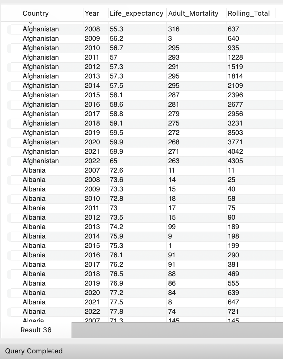
Task 21: We analyze adult mortality trends over time for each country.

Using a window function with SUM() and PARTITION BY Country, we calculate a rolling total of adult mortality across the years. This allows us to observe how mortality accumulates over time and compare it with life expectancy trends, helping to identify patterns such as whether decreasing adult mortality aligns with rising life expectancy.

SELECT 
	Country, Year, Life_expectancy, Adult_Mortality,
	SUM(Adult_Mortality) OVER(PARTITION BY Country ORDER BY Year) AS Rolling_Total
FROM World_Life_Expectancy_Project
;

CONCLUSION & RECOMMENDATIONS

Conclusion:

This project successfully demonstrated how to clean, structure, and analyze a large dataset to uncover meaningful

insights about global life expectancy trends. The cleaning phase ensured data integrity by removing duplicates,

addressing missing values, and standardizing fields, which provided a solid foundation for reliable analysis.

The exploratory phase revealed key patterns:

• Economic factors matter. Countries with higher GDP generally show higher life expectancy, confirming a positive

correlation between wealth and health outcomes.

• Status differentiation. Developed countries exhibit consistently higher life expectancy than developing countries,

though the majority of nations still fall into the developing category, highlighting global health disparities.

• Other health indicators. BMI and Adult Mortality rates also influence life expectancy, reinforcing the

importance of holistic health and lifestyle measures beyond economic strength.

Recommendations:

1. Policy focus on developing nations – Global health initiatives should prioritize developing countries, where

improvements in economic conditions and healthcare infrastructure can drive significant gains in life expectancy.

2. Holistic interventions – Beyond economic growth, efforts should address nutrition (BMI), preventative care,

and reduction in adult mortality through early detection and better health services.

3. Future analysis – Further studies could integrate additional datasets (e.g., education levels,

healthcare expenditure, environmental indicators) to build a more comprehensive understanding of the drivers of

life expectancy.

Overall, this project highlights the value of SQL for end-to-end data analysis—from cleaning and structuring to

exploring correlations and generating actionable insights for decision-making.